
Bayesian Regression in People Analytics
An example of a simple linear regression

I started this post intending to explain why Bayesian approaches are better than the classical statistics methods you were likely taught in your introductory statistics class. But the post got too long so I had to break it up.
So in part 1, I’m giving you an example to compare a Bayesian approach to the frequentist approach (aka those classical methods you learned). I’ll follow this up with another post explaining why Bayesian methods are the methods of the future.
For our example, I will keep it simple with a linear regression. I’ll use the example from Chapter 4 of the excellent regression book by Keith McNulty. Its online version is freely available and provides many practical examples and code to help you learn regression. If you don’t know much about regression, this book is a great place to start.
For this example, let’s look at the relationship between education (education_months is the variable name and is measured in the number of months) and income (annual_income_ppp is annual income adjusted in US dollars). The question we are trying to answer with the data is whether more education is correlated to higher incomes. I recognize there are many other potential factors related to income so let’s roll with this for illustration purposes and not read too much into the conclusion.
Here’s the plot I made using R software that shows the relationship between education and income. I did remove some outlying values where education_months was less than 50 to make the relationship easier to see. The blue line is the classical regression line fit using the frequentist approach and is most likely what you were taught in your introductory stats class. The graph shows a positive relationship. It seems reasonable that more education would be related to higher income.

Let’s fit the model and get the analysis results for this simple linear regression. In R, we do this with the lm function like this:
modelfreq <- lm(annual_income_ppp~education_months, dataset)
The name to the left of the tilde(~) is the y variable (aka dependent variable or response) and the name to the right is the x variable (aka independent variable or input). The default output of this analysis is done with the R command: summary(modelfreq) and gives the following:

There’s a lot here to digest. The key part to notice is the Estimate column where the coefficient for education_months is 451.78. That coefficient is the slope of the regression line. Not surprisingly, because of the graph we did earlier, the coefficient is positive and its associated p-value is 2.2e-16. That tiny number is essentially zero and in the language of classical statistics, is “statistically significant”.
What does that p-value mean? It means it is highly unlikely you could have gotten this result under the assumption that there is no linear relationship between education and income (ie the slope is not zero). And yes, I intentionally use statistical jargon here to explain the result. I find this statement to be a mouthful, which is one reason why I don’t like this approach much. Spoiler alert, I think the frequentist output is harder to explain in simple terms.
To do the Bayesian equivalent in R you would do the following code.
modelbayes <- stan_glm(annual_income_ppp~education_months, dataset, family=gaussian())
Note that you do have to ensure that you have the right R package (rstanarm) installed for this particular code to work. Now compare this code to the previous code. We still have the same tilde with the y and x variables on either side. One difference is that we have to explicitly specify the family=guassian option, which is a fancy way of saying we are assuming a normal distribution. Just as we did with the frequentist approach, the default output of this analysis is done with the R command: summary(modelbayes) and gives the following.
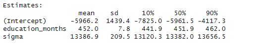
Notice in the mean column the similarity of the estimated intercept (-5966 in the Bayesian approach versus -5937 in the classical approach) and the estimated slope (452 in the Bayesian approach versus 451.8 in the classical approach. Notice also that the standard errors in the classical approach are similar to the sd column (standard deviation) in the Bayesian approach. So your regression equations are pretty similar between the two.
So what is different?
In the classical approach, the focus is on p-values to determine statistical significance. In the Bayesian approach, the focus is on intervals. These intervals are called credible intervals which are different than confidence intervals you may have learned in your stats class. Using the intervals, we would say there is a 10% probability that the slope (education_months) is less than 441.9 and a 90% probability that the slope is less than 462.0. You can do standard probability calculations with these, so I can say that there is an 80% chance that the slope is between 441.9 and 462.0. This interval gives us the conclusion that there is a positive slope and that each additional month of education is related to an increase in annual income of about $450.
Notice the focus of the output is not “Is the slope different from zero?” Rather, the question is simply “What is the slope?” Because there is uncertainty anytime we are using a sample of data to make more general statements, we express that uncertainty in a range of numbers or intervals. Other Bayesian analyses work similarly.
Can you use the Bayesian approach to do what a p-value does? Well, sort of. Looking at the interval for the slope, it is pretty far above zero. So you could say that because the interval doesn’t include zero, it is not likely to have a zero slope representing no relationship. However, there is a fundamental shift in mindset with the Bayesian approach. In the Bayesian approach, we’re not assuming a null hypothesis (slope equal to zero) and then determining whether to reject that hypothesis. We’re simply calculating a range of possible values for the slope, without the need for a null hypothesis.
This interpretation based on intervals works for the other values in the Bayesian output. So there is an interval for the intercept, which doesn’t mean much as it represents the expected income when the months of education is zero. In addition, there is an interval on sigma, which represents the variability around the fitted regression line.
To recap, the goal of a Bayesian approach is not to establish statistical significance but rather the quantification of variability. For this simple example, you get the same conclusions about the positive relationship between education and income.
So why does this matter if you get the same conclusion for the 2 approaches? That is a question for the next post. So stay tuned where I’ll explain all the reasons why I think this Bayesian approach is superior to the frequentist approach you all learned previously. While we’re at it, maybe we can even banish the tortuous language and confusion you got in your Stats 101 class!
If you want to be notified of new articles, you can subscribe for free to this Substack. I aim to post every few weeks and welcome thoughts, questions, and comments.